Characterization of Optical Aberrations Induced by Thermal Gradients and Vibrations via Zernike and Legendre Polynomials ()
Received 15 February 2016; accepted 25 June 2016; published 28 June 2016

1. Introduction
The augmented development of commercial finite element software with the various simulation packages such as thermo-structural static, dynamic and fluodynamic analyses with the use of implicit optimization routines has drastically reduced the designing phase times, cutting down as well the manufacturing costs by eliminating the need to build prototypes and tests, clearly derived from space applications [1] .
Moreover the last decade has witnessed an increasing number of integrated toolboxes not only for space or air-borne but also for ground-based astronomical instrumentation, as for instance the SMI (Structural Modeling Interface Tool), applied to VLTI (Very Large Telescope Interferometer) design [2] or IMAT (I-DEAS Matlab Toolkit) to import nodal model of the structure from FEM into Matlab/Simulink used for the GSMT (Giant Segmented Mirror Telescope), a 30 m class telescope [3] : the aim is the investigation of how cross-coupled perturbations affect the optical performance. In particular wind buffeting and wind force power spectral density, reconstructed via empirical formulas from the wind data, are crucial ingredients for a proper harmonic response analysis.
Even for smaller modules or subunits of instruments coupled to such large structures, we need an analogous procedure passing in both directions the structural data from a FEM code to an integrating platform, in most of the cases MATLAB/Simulink, prone to a correct state-space representation, but can also be Python based if it’s only needed to establish a dialogue with ray tracing program [4] .
Also in our analysis, like in the abovementioned tools, for the specific target of retrieving the Zernike functions to investigate the optical aberrations, it was not necessary to use a dedicated commercial software. Moreover with our implemented tool it is possible automatically to retrieve the nodal displacements from the opticalsurfaces within an harmonic analysis launched in FEM software (ANSYS) and to post-process them isolating in the power spectra in specific amplitudes and phases of interest.
2. FEM Analyses: Thermo-Structural and Harmonic Response
The model under study is a Schwarzschild collimator (SC), setting the proper size of the entrance beam for an optical polarimeter [5] . It has a primary mirror (M1) bonded onto three pads located at the end of three flexure arms, which can be manufactured via EDM technology [6] . Three spokes having a rectangular cross section 10 × 5.5 mm, optimized to reduce the primary mirror obscuration, link the M1 cell to the top ring, holding the secondary mirror (M2). The mirrors, M1 with an outer diameter Ø104 and central bore of Ø18 mm, and M2of Ø16 mm are made of Zerodur, and the supporting structure plus the top ring of Invar 32. Both materials in facts have a very close coefficient of thermal expansion. The primary mirror cell is bolted to a central plate of 40 mm thickness.
Two different scenarios have been simulated:
- A structural analysis with gravity load applied (LC1), at zenith angle z = 75˚, α = 45˚ with α representing the field rotation angle, plus a thermal gradient from 15˚C to 22˚C, uniformly spanned over the entire assembly. The components of the gravity acceleration are the following: ,
,  ,
, . A motor torque of 0.63 Nm is applied to the top ring, mimicking the focuser presence. As external constraints the rim of the central plate has been bonded on three orthogonal planes.
- Modal analysis restricted to the frequency range between 20 and 50 Hz (LC2), including the first 2 eigenmodes, embedded into a harmonic response analysis, where a constant damping ratio ξ = 0.02 has been imposed. Two periodic loads, one due to the presence of a rotary stage motor, the other one associated to a quarter wave retarder plate insertion mechanism have been taken into account. They’re acting along the global z direction, have a phase shift Δφ = 45˚, and their expression is:

Additionally a preload Fb = 500 N of two roller bearings allowing the rotation of the polarization subunit has been also considered (Figure 1).
The nodal displacements over each optical surface are rearranged into the pseudo inverse matrix A+ and by applying the least mean square error the sag and tip-tilt, namely the six rigid body motion values, can be easily retrieved [5] :
 (1)
(1)
where ,
,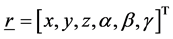 .
.
![]()
Figure 1. Loads distribution with application points and surface relative to the local coordinate system (mainly M1 and M2).
The requirement to fulfill for the tilt angles are Δα, Δβ ≤ 0.1 mrad. Requirements for the yaw angle are much less stringent, and can be 1 mrad, anyway still under definition. Tolerances for the linear displacements are Δx, Δy ≤ 50 µ, Δz ≤ 1 mm. As visible in Table 1, the largest values are reached on M2 because of the high focuser torque.
In the second load case the rotation values are quite modest, if not negligible, and instead a sag effect of M2 towards M1 is more evident, mainly related to the first mode of vibration of the spiders. Spectral distribution of amplitude and phase, for displacement, velocity and acceleration have been determined with peaks corresponding to the first two eigenmodes of 28 and 48 Hz of M1 component (see Figure 2 and Figure 3, Table 2).
3. Zernike Polynomials Fitting
The deformed optical surfaces are consequently fitted via circular Zernike polynomials that, based on the Noll convention [7] , are defined as:
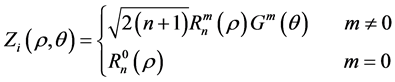 (2)
(2)
where  and
and  are the radial and azimuthal factors:
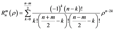 (3)
(3)
 (4)
(4)
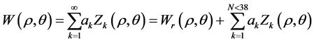
The advantage of using Zernike polynomials over circular and annular apertures is their orthogonality that renders it possible to decompose any wavefront into a sum of independent aberrations. Although orthogonality is fully accomplished only for continuous data [7] , whereas for FEM data is partially lost, we assume anyway that the fitting procedure is suitable because of the homogeneous mesh. Any wavefront can be expressed as an infinite series of Zernike polynomials with coefficients ak given by:
 (5)
(5)
![]()
Table 1. Rigid body motion values for the mirrors M1 and M2 belonging to the SC, relative to the first loads scenario.
![]()
Table 2. Rigid body motion values for M1 and M2 relative to the harmonic case scenario relative to the first eigenfrequency of 28 Hz (see also Figure 2).
![]()
Figure 2. Spectral distribution of the amplitudes vs frequency in the operating range between 20 and 50 Hz for M1.
![]()
Figure 3. Spectral distribution of phase angle vs frequency in the 20 - 50 Hz range for M1.
It’s relevant for our purpose to see how precise the approximation is up to a certain order, usually set to 38, since most of the meaningful aberrations induced by thermal loads and vibrations are within the exploited range. This leads to the estimation of the residual error indicated as![]() . The accuracy is strongly dependent on the grid spacing [8] : a trade-off fitting to both M1and M2 meshes has been found to be (ρ,θ) = 40 × 360. The rms has been used as a proper indicator of convergence versus the increase of the polynomial order, and by the minimal rms it’s possible to estimate the limit of the meaningful primary and secondary aberrations, over which their contribution can be neglected.
. The accuracy is strongly dependent on the grid spacing [8] : a trade-off fitting to both M1and M2 meshes has been found to be (ρ,θ) = 40 × 360. The rms has been used as a proper indicator of convergence versus the increase of the polynomial order, and by the minimal rms it’s possible to estimate the limit of the meaningful primary and secondary aberrations, over which their contribution can be neglected.
The algorithm developed in Python for the determination of the Zernike coefficients converts the nodal Cartesian coordinates of the finite element model to the normalized polar coordinates, applies to them a reverse rigid motion to get back the original reference frame position [9] , employing the following equation:
![]() (6)
(6)
where Rzyz is the Euler rotation matrix, ![]() the deformation values, and
the deformation values, and ![]() are the first three component of the rigid body motion vector. It then projects the coordinates of the meshed data points onto the 40 × 360 uniform grid by a linear interpolation. A polar mask is applied if a central hole is present filtering out the non-existent nodes on the grid. The polynomial coefficients illustrated in Equation (5) are computed by means of the covariance matrix, defined in the following fashion:
are the first three component of the rigid body motion vector. It then projects the coordinates of the meshed data points onto the 40 × 360 uniform grid by a linear interpolation. A polar mask is applied if a central hole is present filtering out the non-existent nodes on the grid. The polynomial coefficients illustrated in Equation (5) are computed by means of the covariance matrix, defined in the following fashion:
![]() . (7)
. (7)
Premultiplying both members by the inverse of the covariance matrix, the coefficients relative to the desired order are obtained. For the sake of clarity in Figure 4 contour plots are illustrated relative to a synthetic surface with 512 × 512 grid where random deformations are applied with a maximum absolute error εmax = 1e−04. As it can be seen in Figure 5 minimal rms is reached at different orders of Zernike polynomials for the two mirrors, depending on the load case: for M2 in both scenarios the rms is smaller than for M1 and for each optical component rms(LC2) < rms(LC1): 3.6545E−07 mm for LC1, 1.73E−08 mm for LC2. In summary, concerning M1 aberrations, under LC1 they can be represented by the first eleven polynomials, namely up to the primary tetra-foil, under LC2 by the first sixteen (primary penta-foil); concerning M2, when LC1 occurs it presents primary trefoil, in LC2 primary astigmatism.
4. Legendre Polynomial Fitting
In the case of rectangular apertures the Zernike polynomials could still be used but their orthogonality is not valid anymore [10] . For this reason 2D Legendre polynomials have been calculated and by least square method the coefficients have been determined as in the Zernike case. The wavefront equation in Cartesian coordinates is given by [11] :
![]() (8)
(8)
with
![]() (9)
(9)
![]() . (10)
. (10)
The best tradeoff number of grid elements selected is 30 × 30, to provide an enough accurate mesh sampling, consisting of 341 nodes for the square entrance surface of the linear polarizing prism. The algorithm is much more sensitive to grid spacing than the Zernike polynomials and it stops after the 5th order, i.e. 36 iterations. The
![]()
Figure 4. First sixteen circular Zernike polynomials, fitting a randomly deformed circular aperture with a grid sampling of 512 × 512 elements. They are numbered following the Noll notation [7] , and in particular can be identified: the piston (N = 1), A- and B-tilt for N = 2, 3, focus (N = 5), pri-coma (N = 9) up to the pri-pentafoil-A, which corresponds to r5cos(5θ).
![]()
Figure 5. All four contour plots are relative to the min rms: in particular the top left one concerns the Z11 for M1 for LC1, top right Z7 for M2 and LC1, bottom left Z16 for M1 at load case 2, bottom right Z6 at load case 2. Load case 2 taken into consideration is relative to 28 Hz, so called first step of the harmonic response analysis.
rms is not lowering down during the simulation but instead presents oscillations. Under the LC1 rmsmin = 7.47793971e−06 and is reached at n = 1, m = 1 (Figure 6 and Figure 7). Another aberration with best fit is reached at n = 1, m = 3. For the vibration analysis the rms error is visibly one order of magnitude smaller with the absolute minimum already reached n = 0, m = 1 with rmsmin = 1.65e−07 and next ones n = 0, m = 3 and n = 2, m = 3.
![]()
![]()
Figure 6. The behaviour of rms error with the variation of n, m orders for LC1 (left) and LC2 (right) for component KALC1.
5. Integration of the Model into the Ray Tracing Software
The final goal, i.e. to seek how perturbation of the wavefront affects image quality, is reached by exporting the Zernike coefficients into Zemax: it consists in inserting them into the so called Extra Data Editor (EDE) immediately above the corresponding lens as a fictitious surface. The maximum number of coefficient allowed is 37 [12] and it’s recommended not to exceed such limit. For the current LC1 analysis Z37 have been implemented respectively for M1 and M2. An offset of 0.05 mm in front of the mirrors has been considered, implying a change in thickness in the lens data editor. The spot size and shape visibly change leading to an increase of the radius from to 83.7 to 108.7 µ and a drastic reduction of the Airy disk diameter from 69.08 down to 13.01 µ (Figure 8).
![]()
![]()
Figure 8. Left: contour plots of the FFT PSF in Zemax [12] , after applying tip-tilt and rigid body motion to all surfaces under scenario LC1, but without taking into consideration the local deformation of the wavefront. Right: PSF under the same conditions but applying Z11 plus Z6 aberrations respectively on M1 and M2. The color bar contains values of the normalized intensity and it’s referred to all wavelengths and a central field.
6. Remarks and Conclusions
In the present work, it has been demonstrated how it’s possible to combine both mechanical FEM analysis and ray tracing software to optimize a set of design parameters for an astronomical instrument subjected to thermal loads and vibrations. The separate outcomes from a thermo-structural static and modal harmonic analyses have been post-processed into Zernike polynomials for circular apertures and Legendre polynomials for the rectangular ones to preliminarily disentangle the optical aberrations they’re affected by. The meaningful surfaces we concentrated on are the primary, secondary mirror collimating the beam from Cassegrain focus with f#11.0 to a 12 mm pencil and the entrance surface to a polarizing beam splitter. In agreement with literature [11] , the minimum rms over the polynomial order has revealed to be a good fitting criterion to establish the most significant aberrations are within the first 37. They’ve been inserted in Zemax into the EDE and consequently the change in PSF on the image plane has been retrieved. With such procedure it’s possible to add up more Zernike coefficients for each surface of interest and determine how PSF and encircled energy are perturbed.
The next step to implement will be to develop a fluid analysis to estimate by the temperature distribution also the variation of the refractive index for air and glasses, in order to investigate which wavefront aberrations are introduced and more precisely also at what distance from the surface they’re located.