1. Introduction
The idea is to test the hypothesis of Mach’s principle by producing a fluctuation in the mass of an object in the lab, use it to produce a steady thrust and match the theory with the experiment [1] -[4] . We push on the object (whose mass is fluctuating) when it is more massive and pull back when it is less massive, this produces a steady linear acceleration, which is detectable in the laboratory. This steady force could be used to produce a propulsive force on a massive object without having to expel propellant from the object. This would be highly desirable from a space rocket point of view, which then would not have to carry a massive payload of expendable fuel.
In Section 2, we give a brief outline of the experimental set up and sample data from the MET. We describe updates to the apparatus and data acquisition system currently under construction. The experimental apparatus is based on a very sensitive thrust balance which is capable of measuring 0.1 microNewton forces. The forces we are currently seeing are in the single digit microNewton range up to approximately 10 - 20 microNewtons maximum.
In Section 3, we present the theory underlying Mach effect thrust. We briefly summarize the work of Dirac 1938 [5] Wheeler and Feynman 1945 [6] and Hogarth 1962 [7] which leads to the development of a new theory of gravitation by Hoyle and Narlikar 1964 [8] -[10] . It appears that the Hoyle-Narlikar (HN) work is fully Machian and incorporates action at a distance via advanced waves as a means to describe the interaction of the universe with a particle here and now. The HN general equation of motion includes mass changing effects which are not present in the usual Einstein geodesic equation. This theory reduces to Einstein’s field equations in the limit of a smooth fluid model of particle distribution and a simple transformation of coordinates to simplify the field equations. The field equations of the new theory start from a simple Machian two body interaction Lagrangian. We address some issues with the HN work, including comments by Hawking [11] in 1965 which have been recently solved by one of us HF [12] .
2. The MET Experiment
The simplest way to test for the presence of matter density fluctuations (see section 3.2) is to subject capacitors to large varying voltage fluctuations. In our case we use a stack of PZT (lead zirconium titanate) dielectric crystals. See Figure 1.
These crystals act as capacitors by storing energy in their dielectric core as they are polarized. The piezoelectric and electrostrictive properties force the crystals to deform (accelerate). The condition that energy vary with time is satisfied as the ions in the crystal lattice are accelerated by the changing external field. These particular Steiner Martin (SM-111) crystals have a dissipation of approximately 0.4% due to heat loss. Note too that simply charging and discharging a capacitor will not produce (Mach effect type) mass fluctuations, only the usual  kind where
  is the internal energy. The capacitor must also be undergoing bulk accelerations of the kind produced by the electrostriction to produce any Mach effect thrust. In the work reported here, the device tested consisted of 8 discs of 2 mm thick by 19 mm diameter PZT crystals glued together with 1 embedded accelerometer. The accelerometer was made with two 0.3 mm thick crystals which are located between the second and third PZT discs near the aluminium end cap. For testing, the crystals were clamped between a thin 4.5 mm
![]()
Figure 1. The Mach effect device is a stack of PZT discs, which are capacitors. Sixteen 1 mm PZT discs were glued together to form the stack. These are then bolted to a reaction mass using 4 - 40 insulated bolts. The electrodes are made from 50.5 μm brass sheet. There are 3 accelerometers present, at the front and back of the stack and one 1/4 way through the stack.
thick aluminium cap and a thicker 16 mm brass disk. The L shaped aluminium mounting bracket was 3 mm thick. The device was bolted inside a Faraday cage which was then attached to the end of a sensitive torsion balance. See Figure 2(a), Figure 2(b) below. The electrodes between the crystal discs are hand cut from sheets of 50.5 μm brass sheet. A stack of brass sheets are clamped together and drilled with holes which helps with adhesion. They are then cut to size and sanded. The glue used is a 50:50 mixture of Versamid 140 and shell Epon Resin 815C. All the positive contacts line up and all the accelerometer electrode positives line up separately and are separately soldered together to form electrode contacts that can be wired for power. For further experimental details of the electronics and calibration methods for the thrust balance we refer the reader to previous works [1] -[4] .
The device was setup as in Figure 1 and Figure 2(a). Figure 2(b) shows a new version of the central column of the thrust balance. It is constructed of 7075 aircraft grade aluminum. Here the Galistan power contacts are central to the column and not offset to the back. We have room for more perspex contacts on the side of the column. If an MET device is operated at constant power, at resonant frequency, it will produce a steady thrust. This particular device had a resonant frequency of 39.3 KHz. Each run consisted of taking data for 32 seconds. The first 6 seconds were quiescent data to establish the background noise. This was followed by 14 seconds of a single frequency 39.3 KHz voltage of around 230 volts, followed by the remaining 12 seconds of quiescent data. Signal averaging was performed by taking a dozen runs under exactly the same circumstances and averaging them to suppress random noise. In order to reduce spurious signals, runs were done with the device facing forward on the balance beam and then also reversed. One can easily reverse the direction by rotation of the faraday cage by 180 degrees. The device is mounted inside the faraday cage on the side wall so this does not affect the device mounting. The mount point is always on the side and is not switched from top to bottom. Once the forward and reversed runs are averaged we take the difference to produce a clear thrust signal where all none reversing spurious thrust signals are eliminated. Two sample data sets of this difference data are shown in Figure 3.
The resonant frequency of the device can be estimated by supplying low power white noise to the device using a SR790 Standford Research two channel signal analyser to show the frequency of impedance dips, and then by trial and error to observe thrust behavior. A sinusoidal voltage of amplitude V = 234 Volts is supplied to the device, which was found to have a resonant frequency of 39.3 KHz or an angular frequency of 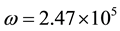 rad/sec. The impedance is taken to be all capacitive. The MET capacitor stack has a capacitance of C = 20 nF. This gives
 . Power is
 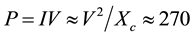 Watts, see Figure 3. The temperature of the thermistor embedded in the aluminum cap and the brass mass are plotted in Figure 3. The scale is not shown but in Figure 4 you can see a plot of the temperature dependence during a typical 14 second pulse. The temperature of the aluminum cap is seen to rise much faster than the brass mass which is also slower to cool.
The temperature change could in principle give rise to an expansion but in previous work we showed how the 6 stainless steel bolts hold the stack under compression, the aluminum and brass expand faster than the PZT so
![]() (a) (b)
(a) (b)
Figure 2. (a) The thrust balance used in the experiment whose results are reported here. C-flex flexural bearing in the central column support the balance beam and provide the restoring torque for thrust measurements. The position of the beam is sensed with a Philtec D63 optical position sensor whose probe is attached to the stepper motor to the left of the damper; (b) New central column for thrust balance, showing central position for the Galistan contacts (Galistan is a Gallium, Indium and Tin alloy which is liquid at room temperatures.) directly between (above and below) the Cflex flexural bearings.
![]()
Figure 3. The red trace indicates thrust, the dark blue trace is the power applied to the device and the light blue trace is the accelerometer. You see 6 seconds of noise followed by the start of the 14 second pulse and then 12 seconds of quiescent data for a full 32 second run. After the switching transient we see a clear thrust of approximately 2 μN and a final transient in the opposite direction when the voltage to the device is switched off. The green trace is the temperature of the thermistor embedded in the brass mass, the magenta trace is the temperature in the thermistor in the aluminum end cap. The scale for temperature are not shown (see Figure 4) but the temperature rise in the aluminum is on the order of 18 degrees Celsius and that of the brass mass is about 8 degrees.
![]()
Figure 4. The figure shows the change in temperature, in the aluminum cap (light blue, dark blue and brown) and brass mass (red, purple and orange), during a typical run consisting of a 14 second power pulse. The cooling times are also indicated. At present the MET has no electronic peltier cooling system, this is a work in progress.
in fact the PZT is compressed and thus heating cannot effect the thrust result, [1] [4] . The effect can also not be caused by any Dean drive vibrations. These could be caused by friction in the bearings of the thrust balance. They would not reverse upon reversing the device, hence they would average to zero and show no net thrust, [1] [3] [4] .
Several upgrades have been implemented at the MET laboratory at CSUF. A new data acquisition system is being tested using Picoscope 4424 and 5242B devices and a data acquisition code has been written in LabVIEW 2013 by one of us, AZ. A smaller vacuum chamber has been set up, with a Hall effect Unimeasure U-80 position sensor. This device and related electronics is described in detail by Woodward, [1] . The U-80 is used to measure thrust vertically. The vacuum system piping has been improved to reduce vibration from the vacuum pump. We have introduced a weighted 4 foot length of 1 inch diameter copper pipe and two verticals and 2 pieces of rubber hose attaching one vertical to the chamber and from the other vertical to the vacuum pump. This significantly reduces the vibration to the chamber from the pump. The power input circuit for the U-80 system has been upgraded with Galistan contacts (for ±voltage and ground) so that vibration, from the external wires, cannot be transmitted to the device inside the Faraday cage, in the vacuum chamber. The Unmeasured U-80 device has been calibrated when it is in a vacuum of 10 mTorr. This was achieved using a weak electromagnet and steel washers with a mass of 0.1 g each. It was possible to drop and pick up 1, 2 and 3 washers at a time during the calibration. The output voltages were stored using a picoscope and averaged. The calibration shows that 0.3 volts is equivalent to 0.1 g = 100 mg. With 100 or more runs averaged together it is possible to get ±1 mg accuracy.
3. MET Theory
In this section we begin with a linearized form of Einstein’s field equations and show how by allowing for mass fluctuations in the equations, Woodward’s mass fluctuation equation [1] -[4] can be derived in a straight forward manner.
Einstein’s early work in 1912, using weak gravitational fields, incorporated Mach’s principle [13] . This involves considering the universe as a simple mass shell with a single particle at the center. As the mass shell universe accelerates the particle is dragged along with it. The same idea was extended to strong gravitational fields by Lynden-Bell [14] . These papers do not go into any detail about the mechanism of the interaction between the universe and the particle. What signals are being sent and what is received? The MET theory of Woodward makes an intellectual stride in assuming there must be a wave-like interaction between particle and universe in order to conserve momentum (between the MET and universe) without giving any details of such. The work of Woodward does cite various authors who have worked on Wheeler-Feynman type absorber theory and it was suggested that advanced waves would allow a particle and the universe to interact in a instantaneous like manner, even though any waves, or signals, between them would still travel at c, the speed of light in a vacuum. The advanced waves however travel at c but backward in time. This is an odd concept but one which correctly describes radiation reaction in electromagnetic interactions (Dirac 1938 [5] ) and can also be used in quantum mechanics as shown by John Cramer [15] -[17] . In quantum mechanics advanced waves can be used very successfully to describe the Einstein Rosen Podolsky (EPR) paradox [18] and quantum eraser [19] type experiments and other forms of entanglement [20] .
In order to go beyond the linearized theory and explain the interaction between the MET device and the rest of the universe, it will be necessary to introduce the electromagnetic radiation reaction theory of Dirac [5] which was given physical interpretation by Wheeler and Feynman 1945 [6] and then applied to gravitation by Hogarth in 1962 [7] and Hoyle and Narlikar in 1964 [8] . The Hoyle-Narlikar theory reduces to Einstein’s theory of gravitation in the limit of matter density being distributed as a smooth fluid. It is a fully Machian theory, by which we mean that the mass of a particle is due solely to its interaction with the rest of the universe. In HN-theory there is no empty universe, that would correspond to no universe, a minimal universe would need at least two particles in it. HN-theory allows for both retarded and advanced waves. The C-field (a scalar field used to create matter) is dropped, particle density can be allowed to change as the universe expands.
3.1. Maxwell Form of Linearized Gravitation
Einstein’s field equations can be linearized and written in a form analogous to Maxwell equations of electromagnetism. Maxwell’s equations in S.I. units are of the form,
 (1)
(1)
where  is the Lorentz gauge, j is current density and
  is charge density and we have E electric and B magnetic fields.
Using the following correspondences from Forward [21] ;
 (2)
(2)
Current I would be  also
also  and
and . Similarly both the vector and scalar potentials are taken to be negative for gravity,
 ![]() and
and![]() . Hence the gravito-electromagnetic (GEM) equations can now be written as:
. Hence the gravito-electromagnetic (GEM) equations can now be written as:
![]() (3)
(3)
where last equation is the Lorentz gauge and we are now taking ![]() to be the mass density as opposed to the charge density in Maxwell’s electromagnetic eqns.
to be the mass density as opposed to the charge density in Maxwell’s electromagnetic eqns.
By substitution of the potentials into the ![]() and
and ![]() equations, the gravitational potentials in S.I. become:
equations, the gravitational potentials in S.I. become:
![]() (4)
(4)
It appears that the gravitational waves travel at ![]() if we are to believe this analogy. But we are fairly confident that gravity waves travel at c so we must make allowance for this. Care must be taken when using this analogy since masses are always seen to attract (locally) and charges can repel or attract, and there are several sign changes for the fields and potentials. Einstein’s gravitational field equations are commonly written as, p154 Weinberg [22] ,
if we are to believe this analogy. But we are fairly confident that gravity waves travel at c so we must make allowance for this. Care must be taken when using this analogy since masses are always seen to attract (locally) and charges can repel or attract, and there are several sign changes for the fields and potentials. Einstein’s gravitational field equations are commonly written as, p154 Weinberg [22] ,
![]()
and the Ricci tensor ![]() has several second derivatives of the metric
has several second derivatives of the metric![]() , see Weinberg or Schutz. In the
, see Weinberg or Schutz. In the
weak field approximation, it is usual to set ![]() where
where![]() . The
. The ![]() is
is
the metric of special relativity or flat space-time.
(Just to clarify notation, Forward uses ![]() when it is more common to use
when it is more common to use![]() . Also
. Also ![]() is used instead of
is used instead of![]() ).
).
We can write Einstein’s equation in the weak field limit, in S.I. units as follows;
![]() (5)
(5)
where![]() . See parametrized post Newtonian (PPN) approximation. This is the basic equation
. See parametrized post Newtonian (PPN) approximation. This is the basic equation
upon which the analogies are based. This can be found in standard text books like Schutz [23] , Weinberg [22] and Misner, Thorne and Wheeler (MTW) [24] .
Starting from the standard definition of the energy stress tensor as defined by MTW [24] page 470, we have proper velocities ![]() and vector pressure P;
and vector pressure P;
![]() (6)
(6)
Take the ![]() term only, and set
term only, and set ![]() for low velocities
for low velocities
![]() (7)
(7)
Now write out Equation (5) for the ![]() time component only, we get,
time component only, we get,
![]() (8)
(8)
Using ![]() for the scalar potential, following Forward [21] we find,
for the scalar potential, following Forward [21] we find,
![]() (9)
(9)
since![]() . Using
. Using ![]() for the vector potential,
for the vector potential,
![]() (10)
(10)
the last equation is identical to the electromagnetic vector potential equation, where![]() . Thus we see that the components of the vector potential
. Thus we see that the components of the vector potential![]() .
.
Forward gives the list of assumptions made in order that the electromagnetic analogy may be applied: [21] [25] .
Normal mass densities, meaning no black holes or neutron stars in the vicinity. All velocities are less than the speed of light in a vacuum and all kinteic energies are non relativistic. The gravitational field is considered weak so that the superposition priciple applies and distances between objects are small so that retardation need not be taken into account.
Unfortunately, the last condition is not very helpful in explaining how the interaction between the particle and universe takes place. The linearized theory is therefore not going to allow us to discuss this interaction, in terms of signals of the advanced or retarded kind, we need to go further. We cannot use linearized theory for a discussion of retarded and advanced waves in the theory of gravitational radiation reaction. The linearized form of gravitation does not have Lienard Wiechert potential equivalents. Even if it did, due to the nonlinear nature of the gravitational field equations the superposition principle would not apply. The theory of Hoyle and Narlikar [8] is a fully relativistic theory based on Mach’s principle, which reduces to the usual Einstein theory when a particle distribution of a smooth fluid is used. The theory requires modification to account for the accelerating expansion of the universe [25] . The C-field (introduced by Hoyle-Narlikar to allow for a steady state universe, corresponding to a mass creation field) is no longer needed. It is interesting to note that the new equation of motion is not exactly a geodesic equation. Hoyle and Narlikar, have mass changing terms in their equation of motion, in a form that reproduces the Woodward mass varying formula.
3.2. Derivation of the Woodward Mass Change Equation
Consideration of the momentum form of the geodesic equation was found by one of us (HF) to lead to Woodward’s mass change formula, by simply allowing the mass to change with time. This method derives the mass fluctuation terms from the temporal part of the d’Alembertian then moves these terms over to the other side of the equation. This requires a slight “fix” and is not fully Lorentz invariant. The same result was obtained independently by a collaborator, Lance Williams, via private communication. HF then discovered the paper by Forward [21] and obtained Woodward’s mass fluctuation formula by extension of that work to allow for mass variation with time. In this paper we outline the simplest possible approach using the momentum geodesic and linearized theory of the last section. The momentum geodesic can be found in the book by Moller, [26] . For a Lorentz invariant approach see Woodard’s book [1] . Starting from the standard definition of the energy stress tensor as defined by [24] Equation (6), where we use proper velocities ![]() and vector pressure P. Take the
and vector pressure P. Take the ![]() term only, and set
term only, and set ![]() for low velocities to give Equation (7). Now write out Equation (5) for the
for low velocities to give Equation (7). Now write out Equation (5) for the ![]() time component only, we get,
time component only, we get,
![]() (11)
(11)
Substitute in the usual flat space term from Equation (9), ![]() and the result for
and the result for ![]() above which gives,
above which gives,
![]() (12)
(12)
This gives the same wave equation, Equation (4), earlier.
We may write the geodesic equation in an equivalent covariant form using momentum as follows, [23] [26] ,
![]() (13)
(13)
![]() (14)
(14)
The equivalent contravariant form for the spatial components gives the equivalent to F = ma,
![]() (15)
(15)
The Christoffel symbols are evaluated as follows:
![]() (16)
(16)
where ![]() is the flat space-time metric and
is the flat space-time metric and ![]() which is different from
which is different from![]() . The time component can be written as,
. The time component can be written as,
![]() (17)
(17)
where ![]() for time dilation and the
for time dilation and the ![]() for low velocities. It is possible to exchange τ for t for low velocities. We have used,
for low velocities. It is possible to exchange τ for t for low velocities. We have used,
![]()
The 4-momentum is![]() .
.
From the temporal form of the momentum geodesic above, rearrange for ![]() as follows,
as follows,
![]()
![]() (18)
(18)
where we have kept the ![]() factor and differentiated it with respect to time. It is important to use the momentum equation so we may introduce a variable mass. The usual geodesic Equation in
factor and differentiated it with respect to time. It is important to use the momentum equation so we may introduce a variable mass. The usual geodesic Equation in ![]() has already cancelled the mass term by considering it a constant of the motion. This is not the case, we must include a
has already cancelled the mass term by considering it a constant of the motion. This is not the case, we must include a ![]() term to account for energy lost by radiation and momentum transfer due to the recoil momentum. There is an equivalent Poynting-Robertson type gravitational radiation reaction of the form
term to account for energy lost by radiation and momentum transfer due to the recoil momentum. There is an equivalent Poynting-Robertson type gravitational radiation reaction of the form ![]() which comes directly from considering mass-energy loss of the system under acceleration. The quantity PR would be the power loss due to radiation.
which comes directly from considering mass-energy loss of the system under acceleration. The quantity PR would be the power loss due to radiation.
Then taking the second derivative of ![]() we have,
we have,
![]() (19)
(19)
where finally we may set![]() , but only after differentiating the
, but only after differentiating the ![]() and neglecting all the velocity terms as before.
and neglecting all the velocity terms as before.
Now substitute Equation (19) into Equation (12) above.
![]() (20)
(20)
which corresponds to Woodward’s mass equation![]() . This is in Woodward’s book [1] p. 85, Equation (A12). Using Woodward’s
. This is in Woodward’s book [1] p. 85, Equation (A12). Using Woodward’s ![]() and
and ![]() where V is volume of the object, we have,
where V is volume of the object, we have,
![]() (21)
(21)
The original derivation can be found in Woodward’s book [1] . Alternate derivations can be found in papers [2] [4] .
3.3. Origin of Mass
The clearest dialogue on mass and its origins can be found in the papers, book and online web article/movies of Frank Wilczek, Nobel Laureate (and Prof at MIT). For layman read his book (which still has physics in it) “Fantastic realities”, p. 236 [27] , for scientists read his paper, [28] . Allow us to quote from p. 236 of the book,
“First; most of the mass of ordinary matter has no connection to the Higgs particle. This mass is contained in atomic nuclei, which are built up from nucleons (protons and neutrons), which in turn are built up of quarks (mainly up and down quarks) and color gluons. Color gluons are strictly massless, and the up and down quarks have tiny masses, compared to the mass of nucleons. Instead, most of the mass of the nucleon (more than 90%) arises from the energy associated with the motion of the quarks and gluons that compose them. According to the original Einstein form of Einstein’s famous equation![]() . This circle of ideas provides an extraordinary beautiful, overwhelmingly positive answer to the question Einstein posed in the title to his original paper [29] , ‘Does the inertia of a body depend on its energy content?’, it has nothing to do with Higgs particles.”
. This circle of ideas provides an extraordinary beautiful, overwhelmingly positive answer to the question Einstein posed in the title to his original paper [29] , ‘Does the inertia of a body depend on its energy content?’, it has nothing to do with Higgs particles.”
Wilczek’s book continues with more points which we summarize below:
Second, for quarks and leptons the Higgs mechanism (field interactions) appear to accommodate mass rather than explain it. We map values of masses and mixings through Higgs field couplings and only have a reliable theory to predict the coupling for the W and Z particles of the weak interaction, not for leptons and quarks.
Third, the Higgs field does not explain the origin of its own mass. A parameter equivalent to the Higgs mass is directly placed into the equation.
Lastly, (again summarizing from Wilczek’s book [27] and his paper [28] ) there is no necessary connection between mass and interaction with any particular Higgs field (Four Higgs particles have been suggested, we have found one, which will do for minimal coupling.) Much of the universe is thought to be made of Dark matter. This Dark Matter does not interact with conventional observational equipment, that includes xray, optical, or radio telescopes. Dark matter is only observed through its gravitational interaction with other nearby ordinary matter. We do not know what this matter is, it could be axions or WIMPs, but because this matter is not visible by conventional telescopes we know it does not interact strongly with photons and probably does not have much of an electro-weak interaction therefore the Higgs mechanism is not involved and is not responsible for the majority of matter in the universe.
This leaves an opportunity to describe the origins of mass in terms of Mach’s principle, which states that the mass of a body is determined by its interaction with the rest of the mass-energy in the universe. However if a body undergoes a sudden acceleration you may ask, “How can the universe respond immediately in a way to conserve momentum?”. In order to explain this we now introduce the concept of advanced waves, which have been used successfully in both classical and quantum physics for the last 70+ years. Advanced waves were introduced by Dirac in 1938 to describe radiation reaction. His radiation reaction force equation is still in use today and can be found in most standard electrodynamics text books. The advanced wave concept was given a physical interpretation by Wheeler and Feynman in 1945 [6] . The idea has since been used successfully in quantum mechanics by John Cramer and later in the theory of gravitation by Hogarth 1962 [7] and Hoyle and Narlikar 1964 [8] whose work we will summarize for convenience below.
3.4. Dirac: Electron Radiation Reaction in Electrodynamics
Dirac [5] first introduced the idea of advanced waves in electromagnetism in order to derive the radiation reaction of an accelerating electron. The idea is as follows, consider a single electron undergoing acceleration. The field surrounding the electron can be thought of in two parts, the outgoing and incoming. The actual field surrounding the electron is the usual retarded Lienard Wiechert potentials and any incident field on the electron.
![]() (22)
(22)
Furthermore, the Maxwell 4-potential wave equation allows for advanced solutions, which are the same form as retarded only they go backward in time (a minus sign on the time component) these also satisfy the wave equation with Lorentz gauge below and![]() .
.
![]() (23)
(23)
We could equally well describe the actual field surrounding the electron by
![]() (24)
(24)
where the ![]() is the total field leaving the electron. The difference between the outgoing waves and the incoming waves is the radiation produced by the electron due to its acceleration.
is the total field leaving the electron. The difference between the outgoing waves and the incoming waves is the radiation produced by the electron due to its acceleration.
![]() (25)
(25)
In the appendix of Dirac’s paper, it is shown that this equation gives exactly the well known relativistic result for radiation reaction which can be found in standard text books on electromagnetism, for example Jackson [30] .
3.5. Wheeler & Feynman: Absorber Theory
Wheeler and Feynman [6] accept Dirac’s result but wish to give a physical explanation as to where the advanced electromagnetic field comes from. They resort to a suggestion made by Tetrode [31] and later by Lewis [32] which was to abandon the concept of electromagnetic radiation as a self interaction and instead interpret it as a consequence of an interaction between the source accelerating charge and a distant absorber. The absorber idea has the four following basic assumptions, which we quote directly from Wheeler-Feynman [6] ,
1) An accelerated point charge in otherwise charge-free space does not radiate electromagnetic energy.
2) The fields which act on a given particle arise only from other particles.
3) These fields are represented by 1/2 the retarded plus 1/2 the advanced Lienard-Wiechert solutions of Max- well’s equations. This force is symmetric with respect to past and future.
4) Sufficiently many particles are present to absorb completely the radiation given off by the source.
Now Wheeler-Feynman considered an accelerated charge located within the absorbing medium. A disturbance travels outward from the source. The absorber particles react to this disturbance and themselves generate a field half advanced and half retarded. The sum of the advanced and retarded effects of all the charged particles of the absorber, evaluated near the source charge give an electromagnetic field with the following properties, [6] ;
1) It is independent of the properties of the absorbing medium.
2) It is completely determined by the motion of the source.
3) It exerts on the source a force which is finite, is simultaneous with the moment of acceleration, and is just sufficient in magnitude and direction to take away from the source the energy which later shows up in the surrounding particles.
4) It is equal in magnitude to 1/2 the retarded field minus 1/2 the advanced field generated by the accelerated charge. In other words, the absorber is the physical origin of Dirac’s radiation field...
5) This field combines with the 1/2 retarded, 1/2 advanced field of the source to give for the total disturbance the full retarded field which accords with experience.
The Wheeler-Feynman paper presents four derivations of the relativistic radiation reaction of an accelerated charge, each successive derivation increasing in generality. The first three derivations proceed by adding up all the electromagnetic fields due to the absorber particles. The fourth is the most general derivation, which only assumes that the medium is a complete absorber and so outside the medium the sum of all the retarded and advanced waves is zero. Each derivation derives the well known relativistic radiation reaction as given in text books, [30] .
So far we have shown that the advanced wave idea has been used successfully in classical physics and now we proceed to show that it can also be advantageously used within quantum mechanics. The transactional interpretation of quantum mechanics was written by John Cramer [15] in the 1980’s. It is a way to view quantum mechanics which is very intuitive and easily accounts for all the well known paradoxes, EPR, which-way detection and quantum eraser experiments. To save space and a few trees we refer the reader to his paper which is a very interesting read. There is also a new book by J. Cramer, “The quantum Handshake, Entanglement, Nonlocality and transaction”, [16] . All the usual quantum results hold and it is simply an alternative point of view from the Copenhagen interpretation and collapsing wavefunction way of thinking.
The previous sections have lead to this point, how to derive the Woodward mass fluctuation formula from a fully covariant relativistic theory which is also fully Machian. In order that a local acceleration get a response from the rest of the universe immediately we need to invoke the advanced wave concept. This would also be required by energy and momentum conservation. Einstein’s linear theory appears to have within it the ability to derive the mass fluctuation but not to explain how the interaction between the accelerating mass and the rest of the universe takes place. This is beyond the validity scope of the linear weak field model. To progress further and to validate the claims made by Woodward [1] , that the MET device interacts via advanced waves with the rest of the universe, we need to turn to Hoyle-Narlikar theory [8] which has Einstein’s general relativity theory incorporated as a special limiting case.
3.6. Hoyle & Narlikar: A New Theory of Gravitation
We begin with a brief overview of Hoyle and Narlikar (HN) theory. This theory is completely equivalent to Einstein’s theory of gravitation in the description of macroscopic phenomenon so all the classical tests apply to both. There are two main differences. In Einstein’s theory the sign of the gravitational constant of proportionality ![]() which appears in the field equations,
which appears in the field equations,
![]() (26)
(26)
is chosen arbitrarily, in HN theory the sign must be negative if all the masses are taken to be positive. Note also that![]() . The second difference is that the equation
. The second difference is that the equation ![]() for an empty universe in Einstein’s theory becomes meaningless in HN theory, in fact it would imply no universe. The HN theory demands that there be at least two particles in a real world, an absorber and an emitter.
for an empty universe in Einstein’s theory becomes meaningless in HN theory, in fact it would imply no universe. The HN theory demands that there be at least two particles in a real world, an absorber and an emitter.
The time symmetry of electrodynamics allows solutions of Maxwell’s equations which are fully retarded or fully advanced or a combination of the two. It is not clear which of these possibilities describes reality. The presence of advanced waves, meaning waves traveling backward in time, was shown by Dirac and Wheeler & Feynman to provide physical real and accurate solutions for radiation reaction for an accelerated charge. HN showed that different cosmologies required either a fully advanced or a fully retarded solution for consistency. Hogarth 1962 [7] discovered that a definite answer could be obtained if the universe was taken to be expanding.
In 1964, Hoyle and Narlikar [8] [33] [34] , derived a new Lagrangian for gravitation which was fully Machian, in a sense that it involved only direct particle interactions. All traditional mass terms were replaced with a direct particle interaction term so that only double integrals remained. The Lagrangian was symmetric so it could be written in terms of half retarded and half advanced mass-waves. This derivation is fully Lorentz invariant. The mass fluctuation terms are not maneuvered into position but appear directly as they should as an addition to the energy-stress part of the field equations. This is exactly the way Woodward intended the mass fluctuation terms to appear. We summarize the HN paper [8] below for convenience.
The three assumptions made about the direct interaction between particles were the following: [8]
1) The mass ma must become a direct particle field, it must arise from all other mass in the universe.
2) Since mass is scalar we expect it to arise through a scalar Green’s function.
3) The action must be symmetric between any pair of particles.
For example, consider a massive particle at point a and sum over all masses in the universe we would rewrite,
![]() (27)
(27)
where ![]() is a coupling constant [33] . Also
is a coupling constant [33] . Also ![]() is a Green’s function with the property
is a Green’s function with the property![]()
![]() . The mass function at a general point X due to particle world line of particle a at point A is defined to be,
. The mass function at a general point X due to particle world line of particle a at point A is defined to be,
![]() (28)
(28)
the mass is allowed to vary from point to point.
![]() (29)
(29)
These two mass equations together with the action below suggest that ma plays the role of inertial mass. These equations incorporate Mach’s principle that the inertia of a particle arises from the rest of the particles (or mass- energy) in the universe [33] . The action (without the electromagnetic field) is given as
![]() (30)
(30)
where![]() . The factor 1/2 comes in because each
. The factor 1/2 comes in because each ![]() is shared by two particles a, b. Using the general wave equation for
is shared by two particles a, b. Using the general wave equation for![]() ,
,
![]() (31)
(31)
where ![]() is a constant which we see will become 1/6 since the wave equation then becomes conformally invariant [9] . Here the g is the determinant of the metric tensor
is a constant which we see will become 1/6 since the wave equation then becomes conformally invariant [9] . Here the g is the determinant of the metric tensor![]() . By methods developed in another HN paper [33] , that is, varying the geometry in a finite volume
. By methods developed in another HN paper [33] , that is, varying the geometry in a finite volume![]() , it can be shown that the variation of the action becomes equivalent to,
, it can be shown that the variation of the action becomes equivalent to,
![]() (32)
(32)
in which ![]() is a symmetric tensor. This formalism becomes a physical theory when we set
is a symmetric tensor. This formalism becomes a physical theory when we set ![]() for all variations of the geometry. This is equivalent to an energy-momentum conservation theorem,
for all variations of the geometry. This is equivalent to an energy-momentum conservation theorem,![]() . These are the field equations of the new gravitational theory from which we may deduce the new equations of motion for a particle. To obtain the equations of motion we consider
. These are the field equations of the new gravitational theory from which we may deduce the new equations of motion for a particle. To obtain the equations of motion we consider ![]() with
with ![]() fixed. The new equation of motion (replacing the old geodesic) becomes,
fixed. The new equation of motion (replacing the old geodesic) becomes,
![]() (33)
(33)
in which ![]() and the Lorentz force has been included on the right hand side for completeness. The right hand side would be zero for no electromagnetism. The gravitational field equations become,
and the Lorentz force has been included on the right hand side for completeness. The right hand side would be zero for no electromagnetism. The gravitational field equations become,
![]() (34)
(34)
where the energy momentum tensor is given by,
![]() (35)
(35)
We have taken greek letters to represent (0, 1, 2, 3) as usual. HN use roman letters for (1, 2, 3, 4) notation and have greek letters for (1, 2, 3). Mass fluctuation terms appear directly in the field equations and in the equation of motion. These are both spatial and temporal. The Einstein theory can be derived immediately from the above in the limit of a smooth fluid approximation for matter distribution and a conformal transformation which is equivalent to a rest frame or COM type frame.
![]() (36)
(36)
The result is the Einstein field equation Equation (26) above, see HN 1964 [8] . The derivative notation is conventional in gravitation but for convenience we state explicitly here; the semicolon refers to covariant derivatives and the comma refers to partial derivative. The covariant derivatives of a vector, co-vector (one-form) and 2nd rank tensor (two-form), in order, are as follows:
![]() (37)
(37)
Since the Hoyle-Narlikar approach uses the European 4-vector numbering (1234) convention, 4 usually being ict the time component needs to change from plus to minus on change from contra- to co-vector in a flat space- time. Also, HN-theory has set c = 1 throughout. In the conformal theory of 1966 [33] smooth fluid approximation alone gives:
![]() (38)
(38)
a further conformal transformation is needed to convert this equation into the Einstein field equations, see [33] 1966 Equations (16)-(20). i.e. Suppose that Equation (38) is a solution for some ![]() and some
and some![]() . Hoyle and Narlikar construct a new solution with
. Hoyle and Narlikar construct a new solution with
![]() (39)
(39)
then under this transformation (where m0 is a constant) Equation (38) becomes:
![]() (40)
(40)
where![]() . This is the Einstein case which requires a “special” conformal frame, with c = 1. The equation takes a simpler form, this is analogous to solving in the rest frame in special relativity. The stress- energy tensor normally used in General Relativity is that for a “perfect fluid” (or ideal gas) in the rest frame of the fluid, see p140 MTW [24] . Mass fluctuations of the fluid cannot show up if you are in the rest frame of the fluid.
. This is the Einstein case which requires a “special” conformal frame, with c = 1. The equation takes a simpler form, this is analogous to solving in the rest frame in special relativity. The stress- energy tensor normally used in General Relativity is that for a “perfect fluid” (or ideal gas) in the rest frame of the fluid, see p140 MTW [24] . Mass fluctuations of the fluid cannot show up if you are in the rest frame of the fluid.
3.7. Woodward’s Mass Change Formula from First Principles HN-Theory
Now in order to connect with the Woodward mass fluctuation formula, we consider the extra terms in Equation (38) alone. Let us rewrite the previous Equation (38) as
![]() (41)
(41)
![]() (42)
(42)
Consider the time component only in a flat space-time using ![]() Taking the Christoffel symbols (of the covariant derivatives) to be zero, and using c = 1 for consistency,
Taking the Christoffel symbols (of the covariant derivatives) to be zero, and using c = 1 for consistency,
![]() (43)
(43)
when we divide by ![]() (which is multiplied throughout in Equation (38)) we get mass fluctuation terms as follows,
(which is multiplied throughout in Equation (38)) we get mass fluctuation terms as follows,
![]() (44)
(44)
Apart from a numerical factor of 4/3, these are the mass fluctuation terms present in Equation (21) and in the book by Woodward, [1] .
Originally in 1964 Hoyle and Narlikar were interested in a steady state cosmology and introduced a C-field to add matter thus keeping the matter density constant during expansion of the universe. This is no longer needed, and here we have not included the C-field in the Lagrangian. The C-field was also not included in their 1964 paper [8] referenced here.
Note that a problem with the HN-theory was pointed out by Hawking [11] in 1965. Hawking agreed that the HN-theory gives Einstein’s equations in the smooth fluid limit and also that the mass-field would be given by half the sum of the retarded and advanced fields. The good news is that this is in effect a boundary condition for the Einstein equations, but the bad news is that it appears incompatible with the expanding universe model because the advanced field would have infinite energy due to expansion. (Retarded waves are red shifted, and advanced waves are blue shifted, due to expansion hence a blue shift divergence.) This problem has been solved by the recent discovery of the accelerating expansion of the universe. This leads to a Rindler horizon which acts as a cutoff for the advanced wave integral and there is no longer a divergence, [12] .
4. Conclusions
It is shown that if Mach’s Principle is taken seriously, and the inertia of a body can be described as the interaction of the body with the rest of the universe, then the advanced and retarded fields transmitted between the particle and the universe can be used to explain the thrust observed in the Mach Effect drive experiments. This idea was originally put forward by one of us, JFW. The idea of inertia being a gravitational effect was first postulated by Einstein. In fact Mach’s principle was the foundation on which Einstein’s general relativity was based. This foundation was later reiterated by Wheeler in his book [35] , where just before page 1 he writes,
Inertia here arises from mass there.
On page 4, Wheeler eloquently comments,
...Therefore every bit of momentum-energy, wherever located, makes its influence felt on the geometry of space throughout the whole universe―and felt, thus, on inertia right here.
This work is an updated version of theory presented at the Joint Propulsion Conference (JPC), hosted by the American Institute for aeronautics and astronautics (AIAA) held in Cleveland Ohio 2014 [25] .
Acknowledgements
One of us, AZ, thanks the Space Studies Institute (ssi.org, Mojave, California), for a research stipend which paid for accommodation and expenses for a summer trip to CSU Fullerton to work on this project 2014. HF thanks the physics department at CSU Fullerton for financial support to present this material at the JPC conference in Cleveland, Ohio 2014.